Problem 1
Step-1
2481-5-2E SA: 8683
SR: 4578
Given that there are n processes to be scheduled on one processor, and the first schedule can be done for any of the n processes, the total numbers of possible schedules in terms of ‘n’ are factorial of n ⇒ n! ( n! = n×n –1×n–2×…×2×1).
For example, for 1 process, there is only one possible ordering: (1), for 2 processes, there are 2 possible orderings: (1, 2), (2, 1). For 3 processes, there are 6 possible orderings: (1, 2, 3), (1, 3, 2), (2, 1, 3), (2, 3, 1), (3, 1, 2), (3, 2, 1). For 4 processes, there are 24 possible orderings. So, for n processes, there are n! possible orderings.
Problem 2
Step-1
Scheduling
The difference between preemptive and non-preemptive scheduling is explained in the table below:
| S. No | Preemptive Scheduling | Non-Preemptive Scheduling |
|---|
- | It interrupts a process in the middle of its execution. | Once a process enters the running state, it is not allowed to be interrupted till it has completed its service time.
- | It takes the CPU away from the process being executed and allocates it to another process with a higher priority. | It makes sure that the process keeps hold of the CPU until it has completed its current CPU burst, thus completing its execution.
- | It is complex to implement. | It is easier to implement.
- | High overhead it produced due to constant switching. | Lower overhead due to simple implementation.
- | The process switches from running state to ready state and then waiting state to ready state. | The process switches from running state to waiting state and then the process terminates.
- | It is costlier to implement due to being complex. | It is cheaper to implement due to being simple.
Problem 3
Step-1
2481-5-17E SA: 8683
SR: 4578
a)
Given data:
Process Arrival Time Burst Time
P1 0.0 8
P2 0.4 4
P3 1.0 1
Step-2
If the processes arrive in the order p1, p2, p3, and are served in FCFS order, the result shown in Gantt chart, which is a bar chart that including start and finish times of each of the participating processes:
| P1 | P2 | P3 |
|---|
0 8 12 13
The Formula’s are:
Turnaround time(Pi) = Completion Time(Pi) – Arrival Time(Pi) n Average Turnaround time = 1/n ∑ (Ci – Ai) i=1 where Ci is Completion Time(Pi) and Ai is Arrival Time (Pi)
Average Turnaround time = 1/3[(8-0) + (12-0.4) + (13-1) ]
= 1/3[8 + 11.6 + 12]
= 1/3[31.6]
= 31.6/3
= 10.53
Therefore, the Average Turnaround time with FCFS algorithm =10.53
Step-3
b)
**** Using SJF scheduling, we would schedule the processes according to the following Gantt chart:
| P1 | P3 | P2 |
|---|
0 8 9 13
Average Turnaround time = 1/3[(8-0) + (13-0.4) + (9-1)]
= 1/3[8 + 12.6 + 8]
= 1/3[28.6]
= 28.6/3
= 9.53
Therefore, the Average Turnaround time with SJF algorithm=9.53
Step-4
c)
Using future –knowledge scheduling algorithm, we would schedule the processes according to the following Gantt chart:
| P3 | P2 | P1
---|---|---|---
0 1 2 6 14
Average Turnaround time = 1/3[(14-0) + (6-0.4) + (2-1) ]
= 1/3[14 + 5.6 + 1]
= 1/3[20.6]
= 20.6/3
= 6.87
Therefore, the Average Turnaround time with future-knowledge algorithm = 6.87
Problem 4
Step-1
2481-5-4E SA: 8683
SR: 4578
The advantage of having different time-quantum sizes at different levels of a multilevel queuing system is processes that need more frequent servicing for instance, interactive processes such as editors, can be in a queue with a small time quantum. Processes with no need for frequent servicing can be in a queue with a larger time quantum, requiring fewer context switches to complete the processing, making more efficient use of the computer.
Problem 5
Step-1
CPU Scheduling Algorithms
a. The relationship between priority and SJF or Shortest Job First is that the shortest job has the highest priority and is served first.
Step-2
b. The relationship shared between Multilevel Feedback Queues and FCFS or First Come First Serve is that the lowest level of Multilevel Feedback Queues is First Come First Serve.
Step-3
c. The relationship between priority and FCFS or First Come First Serve is that First Come First Serve assigns the highest priority to the job that has been in existence the longest time, thus serving the job that came first before the others.
Step-4
d. There is no relationship between the two scheduling algorithms RR or Round Robin and SJF or Shortest Job First. RR is a preemptive scheduling algorithm whereas SJF is a non-preemptive scheduling algorithm.
Problem 6
Step-1
2481-5-10E SA: 8683
SR: 4578
The I/O-bound processes would spend more time waiting for I/O than using the processor. So, they usually have used less CPU time in the recent past than other process. As soon as they are done with an I/O burst, they will get to execute on the processor. So this algorithm will favor I/O bound programs.
CPU-bound programs would spend more time on executing programs than I/O. However, since the algorithm takes into account only recent history, the CPU bound processes will not starve permanently. If a process has been prevented from using the processor for some time, it becomes one of the processes that have the least CPU time(=0) in the recent past and eventually it will get a chance to use CPU.
Problem 7
Step-1
Scheduling
The difference between Process Contention Scope or PCS scheduling and System Contention Scope or SCS scheduling is explained in the table given below:
| S. No | PCS Scheduling | SCS Scheduling |
|---|
- | PCS scheduling is performedwithin the process. That is local to the process. | SCS scheduling is carried outon the operating system with kernel threads.
- | PCS involves the thread library scheduling threads onto available Light Weight Processes. | In SCS scheduling, the system scheduler scheduling kernel threads to operate on single or multiple CPUs.
- | On systems implementing many-to-one and many-to-many threads, PCS occurs, as competition occurs between threads that are part of the same process. | Systems employing one-to-one threads use only SCS.
- | In Pthread scheduling, PTHREAD_SCOPE_PROCESS schedules threads by using PCS Scheduling, by scheduling the user threads onto attainable LWPs, using the many-to-many model. | In Pthread scheduling, PTHREAD_SCOPE_SYSTEM schedules threads by using SCS Scheduling, by connecting user threads to specific LWPs, effectively employing a one-to-one model.
Problem 8
Step-1
Threads
Y es it isimportant to bind a real-time thread to a light weight process (LWP). By doing so, there will not be any latency while waiting for an accessible light weight process and the real-time user thread can be scheduled rapidly. If a real-time thread is not bound to an LWP, then the user thread may have to fight for an available LWP before being scheduled.
Problem 9
Step-1
Consider the data for the three processes and the recent CPU usage are as follows:
| S. No | process | Recent CPU usage |
|---|---|---|
| 1 | P1 | 40 |
| 2 | P2 | 18 |
| 3 | P3 | 10 |
Formulae to compute priority is as follows:

Step-2
Compute the priorities for each process as follows:
• For process P1, substitute the recent CPU usage as 40 and base is 60:

• For process P2, substitute the recent CPU usage as 18 and base is 60:

• For process P3, substitute the recent CPU usage as 10 and base is 60:

Step-3
From the above data the priorities for the three processes P1, P2, and P3 are 80, 69 and 65 respectively.
Here process P1 has the highest priority, P2 is the next priority and P3 has the lowest priority.
In traditional Unix scheduler the process priority is dynamic. The priorities are raised or lowered depends on the CPU interval time to execute a process by adjusting the priorities dynamically.
Hence, from the above information the first process is ready for execution which has highest priority, but the CPU time is 40(higher compared to other process). So, scheduler cannot wait longer time to wait for the first process execution, So, the priorities are lowered.
Problem 10
Step-1
Importance of distinguish I/O-bound and CPU-bound programs
The scheduler need to distinguish I/O (Input/Output) – bound programs from CPU (Central Processing Unit) – bound programs for efficient use of computer resources. The scheduler efficiency depends on the optimum utilization of CPU. This can be achieved by observing the properties and distinguishing the programs.
I/O-bound programs utilize small amount of CPU resources. They have the property of performing small amount of computations before performing IO. This property makes I/O-bound programs not to use their entire CPU quantum.
CPU-bound programs utilize large amount of CPU resources. They have the property of performing computations without performing any blocking IO operations. This property makes CPU-bound programs to utilize their entire CPU quantum.
Based on these properties of I/O-bound and CPU-bound programs, scheduler should distinguish and give priorities. Scheduler should give high priority to I/O-bound programs. It should allow I/O-bound programs to execute before the CPU-bound programs. This scheduling will help in better utilization of computer resources.
Problem 11
Step-1
CPU utilization and response time:
• Generally, CPU utilization should be maximized and response time should be minimized.
• CPU utilization can be maximized by minimizing the time spent in context switching, as the CPU is idle during context switching.
• The time taken from the submission of request to time the first response is produced is called the response time.
• When context switching is done rarely, then it would indeed result in decrease in the response time.
Step-2
b.
Average turnaround time and maximum waiting time:
• Generally, average turnaround time and average waiting time should be minimized.
• The interval from the time of submission of a process to the time of completion of a process is the turnaround time.
• Turnaround time is the time spent by a process waiting to get into memory, waiting in the ready queue, executing on CPU, and doing I/O.
• Waiting time is the time spent by a process waiting in the ready queue.
• The average turnaround time can be minimized by executing the jobs with shortest CPU bursts.
• If the jobs with shortest CPU bursts are executed first, then it will indeed increase the waiting time of the jobs with large CPU bursts and thus it will maximize the waiting time.
Step-3
c.
I/O device utilization and CPU utilization:
• Jobs can be categorized into CPU bound jobs and I/O bound jobs.
• I/O bound jobs spend most of the time using I/O devices and spend less time doing computation using CPU.
• CPU bound jobs spend most of the time doing computation using CPU and spend less time using I/O devices.
• CPU utilization can be maximized by executing CPU bound jobs that have large CPU bursts.
• I/O device utilization can be maximized by executing I/O bound jobs. As soon as the I/O device is free, it can be allocated to an I/O bound job.
Problem 12
Step-1
Lottery ticket are based on the probabilistic scheduling algorithm in which each processor are provided with some number of lottery tickets and scheduler make decision of picking next process by drawing random ticket.
Step-2
Since every process are assigned a lottery ticket so if higher-priority processes are assigned more tickets, than the BTV scheduler can assure that threads which are higher priority gain more consideration from the CPU than threads that have lower priority. The reason behind is that the process which have more tickets has higher probability of getting the CPU.
Problem 13
Step-1
There are two ways for maintaining a queue of processes for a processor:
• Processing core having its own run queue
• All processing core sharing single run queue
Step-2
Processing core having its own run queue: In this method each CPU works on its own local run queue. A processor can takes the process directly from queue.
Advantages:
• The processes present on the run queue are evenly distributed across the processor maintaining that run queue. This is known as load balancing.
• There is no interference or conflict even if two or more processors are making use of a scheduler simultaneously.
• At the time of making decision for a processing core, scheduler only requires to look at its local run queue.
Disadvantages:
• Extra required for maintaining different queue for different processor.
• Each processor has its own queue so when some processor’s queue get completely empty then that processor get idle where as it might be possible that other processors are busy.
Step-3
All processing core sharing single run queue: In this method there is only one run queue which is shared by all CPU. Whenever any process assign a processor then process is taken from shared queue.
Advantages :
• This method leads to better utilization of processor.
• Any CPU that is idle can extract a runnable process from the common run queue and executes it.
• No extra work is required for maintaining different queue for different processor.
Disadvantages:
• There is load balancing problem in shared queue method.
• When there are different run queues, this can even lead to deadlock state if not protected with any locking scheme.
Problem 14
Step-1
The formula to predict the length of the next CPU burst is as follows:

a.
Given  and
and  .
.
Substitute  in equation (1).

So, when  and
and  , the prediction for the next CPU burst will be 100 ms.
The recent history has no effect (current conditions are assumed to be transient).
Step-2
b.
Given  and
and  .
.
Substitute  in equation (1).

So, when  and
and  , the prediction for the next CPU burst depends more on the most recent behavior of the process and less on the past history of the process.
Problem 15
Step-1
A CPU bound process is one which has more CPU bound operations and an I/O bound process is one which has more of I/O bound operations.
• In the given scheduling algorithm, each process has initial 50 milliseconds of time quantum and a priority.
• So, if a process utilizes all of its time quantum, then 10 milliseconds more are assigned to it and its priority is also increased. This type of process is CPU bound process.
• On the other hand, when a process blocks for I/O before utilizing its full-time quantum, then its time quantum is reduced by 5 milliseconds but the priority remains same. This type of process is I/O bound process.
• It can be induced that after completion of each round, a CPU bound process gets more time quantum for execution and its priority is also increased.
Step-2
Hence, a regressive round-robin scheduler favors CPU-bound processes.
Problem 16
Step-1
Turnaround time is the total time taken by process from submission to its completion.
Waiting time is the time spent by process in ready queue for getting the processor.
The burst time and priority of each processor is given below as:
| process | burst time | Priority |
|---|---|---|
| P1 | 2 | 2 |
| P2 | 1 | 1 |
| P3 | 8 | 4 |
| P4 | 4 | 2 |
| P5 | 5 | 3 |
Step-2
FCFS algorithm : It Stand for First Come First Serve. In this, the process which comes first execute first, come second execute next.
Gantt chart for FCFS algorithm:
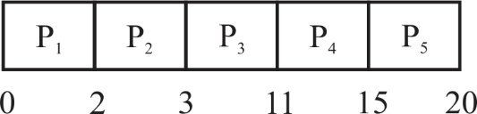
In the above Gantt chart processes arrive in the order P1, P2, P3, P4 and P5.
SJF algorithm : It stands for Shortest Job First. The process which has least burst time execute first the second least execute second and so on.
Gantt chart for SJF algorithm:
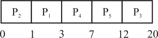
In the above Gantt chart processes when there is availability of CPU it is assigned to the processes.
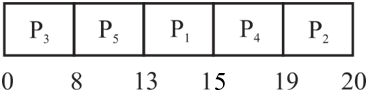
Non- preemptive priority algorithm : The process having highest priority showing with largest number execute first and showing second largest number execute second and so on.
Gantt chart for Non- preemptive priority algorithm:
Round robin algorithm: It works on time quantum.
Gantt chart for round robin algorithm with quantum=2
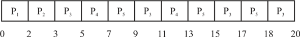
In the above Gantt chart each processes is interrupted after time slice of 2 quanta.
Step-3

Turnaround time of each processor in FCFS:
| process | Turnaround time |
|---|---|
| P1 | 2 |
| P2 | 3 |
| P3 | 11 |
| P4 | 15 |
| P5 | 20 |
Turnaround time of each processor in SJF:
| process | Turnaround time |
|---|---|
| P1 | 3 |
| P2 | 1 |
| P3 | 20 |
| P4 | 7 |
| P5 | 12 |
Turnaround time of each processor in Non-preemptive priority:
| process | Turnaround time |
|---|---|
| P1 | 15 |
| P2 | 20 |
| P3 | 8 |
| P4 | 19 |
| P5 | 13 |
Turnaround time of each processor in Round Robin:
| process | Turnaround time |
|---|---|
| P1 | 2 |
| P2 | 3 |
| P3 | 20 |
| P4 | 13 |
| P5 | 18 |
Step-4
 .
.
Waiting time of each process in FCFS:
| process | Waiting time |
|---|---|
| P1 | 0 |
| P2 | 2 |
| P3 | 3 |
| P4 | 11 |
| P5 | 15 |
Waiting time of each process in SJF:
| process | Waiting time |
|---|---|
| P1 | 1 |
| P2 | 0 |
| P3 | 12 |
| P4 | 3 |
| P5 | 7 |
Waiting time of each process in Non-preemptive priority:
| process | Waiting time |
|---|---|
| P1 | 13 |
| P2 | 19 |
| P3 | 0 |
| P4 | 15 |
| P5 | 8 |
Waiting time of each process in Round Robin:
| process | Waiting time |
|---|---|
| P1 | 0 |
| P2 | 2 |
| P3 | 12 |
| P4 | 9 |
| P5 | 13 |
Step-5


SJF algorithm has the minimum average waiting time of 4.6.
Problem 17
Step-1
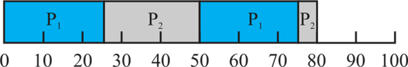
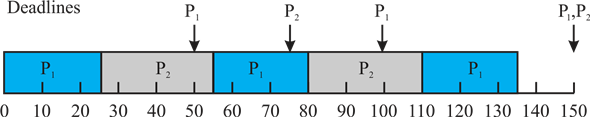
• It is given that Preemptive and round robin algorithm is used to schedule the process and each process has given a priority value. If there is no process to run then the task is taken as P idle.
• According to Preemptive algorithm , if any process is running and any other higher priority comes into existence then the running process is preempted by higher priority process.
• Round Robin scheduling algorithm is based on the time quantum. The process will be provided to CPU by mechanism first come first serve. After processing each process at once with time quantum, the sequence will be repeated.
Step-2
Scheduling order of the process using Gantt chart is given below:

Explanation of above Gantt chart:
• In time interval 0 to 20: will execute in this slot as arrival time of
  is 0 and no other process has arrived during the time slot.
• In time interval 20 to 25: No process will execute as  already completed and no other process is available in ready queue.
• In time interval 25 to 35: will execute.
• In time interval 35 to 45: will execute.
• In time interval 45 to 55: will execute.
• In time interval 55 to 60: will execute.
  will be preempted as process
  with priority higher than
  has arrived.
• In time interval 60 to 75: will execute.
• In time interval 75 to 80: will execute.
• In time interval 80 to 90: will execute.
• In time interval 90 to 100: No process will execute as ,
, ,
, 
 already completed and no other processes are available in ready queue.
• In time interval 100 to 105: will execute as no other process available at this moment.
• In time interval 105 to 115:  will execute because it has more priority then
 .
.
• In time interval 115 to 120: will execute as****
 has completed its burst time.
Step-3
Turnaround time is the total time taken by process from submission to its completion.
 .
.


Step-4
c.
Waiting time is the time spent by a process waiting in the ready queue.
Waiting time for 


Step-5
d.
CPU utilization can be calculated as given below:

Problem 18
Step-1
Nice value is used to provide a specific priority to the process at the time of invoking or calling.
• The default nice value is 0.
• The limits of nice value are -20 to +19.
• A lower nice value indicates a higher priority. It means -20 indicates a highest priority.
• A higher value indicates a lower priority. It means 20 or 19 shows the lower priority.
• A higher priority process is always assigned more CPU time than a low priority process.
Step-2
The non- root processes are allowed to assign nice values greater than or equal to zero.
• If the non- root processes are allowed to assign nice values less than zero, then all the non- root processes will provide themselves a higher priority.
• Then there will be an issue to which non-root processes the CPU is to allocated as they are all of high priority.
Hence, the root user can only be allowed to assign nice values less than zero.
Problem 19
Step-1
Starvation due to scheduling algorithms
First – come, first – served (FCFS) algorithm : This scheduling algorithm allocates the CPU (Central Processing Unit) resources to the process that requests the resources first.
Shortest – Job – First (SJF): This scheduling algorithm allocates the CPU (Central Processing Unit) resources to the process that has the smallest CPU burst.
Round – robin : This scheduling algorithm allocates the CPU (Central Processing Unit) resources to each of the process in the circular queue for a time interval of up to 1 quantum (Time quantum is a small amount of generally from 10 to 100 milliseconds).
Priority Scheduling : This scheduling algorithm allocates the CPU (Central Processing Unit) resources to the process that has the highest priority (a priority is associated with each process).
Among all the four scheduling algorithms Shortest – Job – First and Priority scheduling could result in starvation.
Step-2
In the Shortest – Job – First scheduling algorithm, the longest job will be in the indefinite blocking or starvation. Starvation arises when shortest jobs keep on arriving before the current shortest job completes its execution. In this case, the shortest job is always available to execute and longest job will starve.
In the Priority scheduling algorithm, the lowest priority job will be in the indefinite blocking or starvation. Starvation arises when highest priority job keeps on arriving before the current highest priority job completes its execution. In this case, the highest priority job is always available to execute and low priority job will starve.
Therefore, Shortest – Job – First and Priority scheduling could result in starvation.
Problem 20
Step-1
a)
• ****If the two pointers referred to the same process in the ready queue using Round Robin scheduling Algorithm, the process priority get increased every time.
• This phenomenon also called receiving preferential treatment.
• Preferential treatment means take the advantage over the other process in the ready queue which are having more priority.
Consider the two pointer p 1 and p 2 have the same references to the Process P 1 and these two pointers are put in the ready queue at time quantum t.
Then each process gets ½ = 50% of CPU time with at most ‘t’ time units.
Each process waits for maximum time i.e (2-1)xt time unit until its next time quantum.
Step-2
b)
The two-major advantage of this preferential treatment scheme is as follows:
• In the Process control block, the CPU can give high priority to the Important processes. Hence, the important process will complete the job first.
• Higher Priority in the received treatment.
The Disadvantages**** preferential treatment are as follows:
• Shorter jobs will suffer to wait in the ready queue for its execution.
• Less Priority.
Step-3
c)
The best advice to modify the RR algorithm to avoid this issue without the duplicate pointers is allot a longer amount of time to processes deserving higher priority.
It means provide various time quantum to complete the jobs one after the other in the RR scheduling algorithm.
Problem 21
Step-1
Given data:
• Number of I/O bound tasks=10
• Number of CPU bound tasks=1
• Time taken for context-switching=0.1 millisecond
Time quantum is 1 millisecond:
The CPU bound job will be preempted after the time quantum of 1 millisecond.
The I/O bound job will execute for 1 millisecond and after that context switching takes place.
When the time quantum is 1 millisecond, there will be 0.1 units of context switch for both CPU and I/O bound jobs.
Hence, the CPU utilization 

Step-2
Hence, the CPU utilization when the time quantum is 1 millisecond is 91%****.
Step-3
The time quantum is 10 milliseconds:
The CPU bound job will be executed for 10 milliseconds and then context switch takes place. The CPU bound job will not be preempted for 10 milliseconds.
Therefore, the time taken for a CPU bound job will be 10+0.1=10.1 ms.
The I/O bound job will take 10 milliseconds to complete. The I/O bound job will perform a context switch once for 1 millisecond. This is because it issues an I/O operation for every 1 millisecond of CPU utilization.
Therefore, the time taken for an I/O bound job will be 1ms + 0.1ms =1.1 ms.
As there are 10 jobs, the time taken for ten I/O bound jobs will be  .
.
Hence, the CPU utilization 

Hence, the CPU utilization when the time quantum is 10 millisecond is 95%****.
Problem 22
Step-1
One possibility:
If the program uses only a large fraction of its time quantum and not the entire time quantum, thereby increase of priority associated with that process, The program could maximize the CPU time allocated to it by not fully utilizing its time quantums.
Another Possibility:
Round Robin Scheduling: A multilevel queue scheduling algorithm partitions the ready queue in several separate queues. The processes are permanently assigned to one queue, based on memory size, process priority, process type.
Breaks a process up into many smaller processes and dispatch each to be started and scheduled by the operating system. Separate queue might be used for foreground and background processes. Foreground queue might be Round Robin where as background may be FCFS algorithm.
Problem 23
Step-1
(a)

 is the rate of change of priority when the process is running
 is the rate of change of priority when the process is waiting
0 is the rate when the rate when the process entered in ready queue.
• From the above question, all the processes having initial priority of 0 when it is entered into the ready queue.
• The priority is increased when the process is running from the ready state at the rate  which is greater than 0. Therefore, the highest priority of the process is
  .
.
• When the highest priority process is running (the first processes which entered into the ready queue), its priority is increasing at a rate ( ). Therefore, no other processes will preempt until its completion.
• As the highest priority processes running is higher than the processes which are waiting, it seems to be a First-Come-First-Serve (FCFS) algorithm. The processors which are waiting for a long time will be run and its priority is increasing. __
Hence, the algorithm results from the equation are FCFS.
Step-2
(b)

• As the highest priority processes are running, no other processes which are in the ready queue will not preempt the running process. Therefore, its priority is decreasing at a rate  .
.
• But, the process can be preempted by the new processes because when the new process enters into the ready queue, its initial priority is 0. The 0th priority is greater than the priority of the waiting process  .
.
Therefore, the last come process is served first. Therefore, the algorithm results from the explanation is LIFO (Last In First Out).
Problem 24
Step-1
(a) FCFS —discriminates against short jobs since any short jobs arriving after long jobs
will have a longer waiting time.
Step-2
(b) RR —treats all jobs equally (giving them equal bursts of CPU time) so short jobs will
be able to leave the system faster since they will finish first.
Step-3
(c)Multilevel feedback queues —work similar to the RR algorithm—they discriminate
favorably toward short jobs.
Problem 25
Step-1
Windows scheduling algorithm uses 2 type of scheduling algorithm, one is priority based scheduling and preemptive scheduling algorithm.
There are 6 priority classes given below as:
• IDLE_PRIORITY_CLASS
• BELOW_NORMAL_PRIORITY_CLASS
• NORMAL_PRIORITY_CLASS
• ABOVE_NORMAL_PRIORITY_CLASS
• HIGH_PRIORITY_CLASS
• REALTIME_PRIORITY_CLASS
The values can be: IDLE, LOWEST, BELOW_NORMAL, NORMAL, ABOVE_NORMAL, HIGHEST, TIME_CRITICAL.
Step-2
A thread in the REALTIME_PRIORITY_CLASS with a relative priority of NORMAL is 24 (given from figure 6.22).
Step-3
A thread in the ABOVE_NORMAL_PRIORITY_CLASS with a relative priority of HIGHEST is 12 (given from figure 6.22).
Step-4
A thread in the BELOW_NORMAL_PRIORITY_CLASS with a relative priority of ABOVE_NORMAL is 7 (given from figure 6.22).
Problem 26
Step-1
• The combination of REALTIME_PRIORITY_CLASS and TIME_CRTICAL priority provides the highest possible relative priority that is 31.
• Assume there is no threads belong to the REALTIME_PRIORITY_CLASS and that none may be assigned a TIME_CRTICAL priority.
• If above condition is true then a combination of HIGH_PRIORITY_CLASS and HIGHEST priority within that class with a numeric priority of 15 corresponds to the highest possible relative priority in Windows scheduling (According to figure 6.22).
Problem 27
Step-1
Time quantum is also known as time slice. It is small unit of time. Time quantum is used in time sharing system.
Time quantum and priority are inversely proportion to each other. Higher priority refers lesser the time quantum and vice versa.
Step-2
According to the Solaris operating system for time sharing needs the time quantum (in milliseconds) for a thread with priority 15 is 160 and for a thread with priority 40 is 40 (according to figure 6.23).
Step-3
A thread with priority 50 has used its entire time quantum without blocking, so the scheduler will assign a new priority to this thread that is 40 (according to figure 6.23).
Step-4
A thread with priority 20 blocks for I/O before its time quantum has expired, so the scheduler will assign a new priority to this thread of 52 (according to figure 6.22).
Problem 28
Step-1
CFS stands for Completely Fair Scheduler and it is default linux scheduling algorithm. Priority value is not provided directly by the CFS scheduler but it maintain the virtual run time of each task by pre-task variable vruntime which provide the runtime of each process.
Lower nice value shows higher priority and higher nice value shows the lower priority. A higher priority process is always assigned more CPU time than a low priority process.
Step-2
When both tasks A and B are CPU bound and nice value of A and B is given as -5 and +5 respectively then vruntime will be small for task A than task B as -5 for task A indicates a higher priority than task B.
Step-3
When task A is I/O bound and B is CPU bound, the vruntime will be smaller for task A than task B because task A has high priority and I/O bound process will run shortly before blocking for another I/O.
Step-4
When task A is CPU bound and task B is I/O bound the vruntime of task A will be less than value of vruntime of task B as CPU bound process will consume its time period whenever it will run on processor and it can be preempted by I/O bound.
Problem 29
Step-1
InProportional share scheduler, some CPU time is previously allocated to each processor and every job contains certain weight. And on the proportion of the weight, each job gets the part of available resources.
Step-2
A priority inversion problem is one in which a resource required by a high priority process is being acquired by a low priority process and that has preempted by medium priority process.
Due to which the highest priority process cannot be implemented before the medium priority process and lower priority process.
Example: A and B are 2 processes A has higher priority than B and B acquire an exclusive shared resource that is required by the A. let C be a medium priority that comes into existence. If B is running, A and C is blocked.
B can be preempted by C as it has higher priority. But A cannot run before B as A needs that resource which is acquired by B. So the priority of A and B is inverted.
Step-3
The solution to this problem is that a high priority process and a low priority process should interchange their priorities only till the high priority process completes its work with the resource, after that priorities can be same as initial.
This can be a solution which can be implemented within the context of a proportional share scheduler.
Problem 30
Step-1
Rate-monotonic scheduling is the scheduling algorithm which is used today in real-time operating system. In this static-priority scheduling class is being used. In case of static-priority scheduling class if the duration of the cycle is short then priority of the job will be higher.
Earliest - deadline – first scheduling places a process in priority queue which is having a due deadline that means the process which is near its deadline given the highest priority, whereas rate-monotonic scheduling places a process in priority queue having shorter period which leads to higher priority.
Step-2
Circumstances where rate-monotonic scheduling algorithms are inferior in comparison to the earliest-deadline first scheduling algorithm in meeting the processes are as follows:
• In case of static priority assignment rate monotonic is preferred whereas in case of dynamic priority assignment earliest deadline first assignment is preferred.
• When tasks-sets with the higher processor utilization is required then in that situation Rate-monotonic scheduling algorithm is not preferred.
Problem 31
Step-1
Rate-monotonic scheduling places a process in priority queue having shorter period which leads to higher priority. It plays an important role in real time as it guarantee that the tasks are basically schedulable. The tasks which is meeting their deadline in a proper time is said to be schedulable.
Consider the following Gantt chart:
Explanation of the Gantt chart:
• Process has the shorter period so it will be scheduled first at time
 . Its burst will finish at
 , giving the CPU to process
 .
.
• This process will get to execute till the end of the deadline for process at
at , upon which it will get preempted.
• Thus process got to execute for
 . Process
 will execute till
 .
.
• This is the deadline for process but it still needs
 to complete its burst.
Hence, it can be said that the 2 processes cannot be scheduled by rate-monotonic scheduling.
Step-2
Earliest-deadline-first scheduling places a process in priority queue which is having a due deadline that means the process which is near its deadline given the highest priority.
Consider the following Gantt chart:
Explanation of the Gantt chart:
• These two processes can be scheduled with earliest-deadline-first scheduling. Scheduling will start with process since it has the earliest deadline
 .
.
• Process will be scheduled in at
 . It will not get preempted by process
 at
at as it has the earlier deadline, that is
 .
.
• It will relinquish control of the CPU at the end of its burst, at .
.
• At this point, process will be scheduled in. It too will execute till its burst’s end, till
 .
.
• At this time, process will be scheduled in as process
 ’s deadline has been met. It will not be preempted by process
 at
at as both the processes’ deadlines are the same, that is
 .
.
• Process will get the CPU at
 . Its burst will finish at
 , where the CPU will remain idle till
 .
.
Hence, it can be said that the 2 processes can be scheduled by earliest-deadline first scheduling.
Problem 32
Step-1
A hard real time system is one in which a process is serviced within a given deadline or time.
The performance of the hard real time systems is affected by the interrupt latency and dispatch latency.
Step-2
Interrupt latency is the amount of time between the occurrence of the interrupt to the CPU and the first respond of the CPU to the interrupt.
For a hard real time system, Interrupt should be bounded as the CPU has to first complete the currently running instruction, save its state and then the interrupt will be serviced by ISR (Interrupt Service routine) which will check what type of interrupt has been occurred.
It is very important in real operating system to reduce the interrupt latency because if interrupt latency is reduced, it will be ensured that the real time system get immediate attention.
Step-3
Dispatch latency is the amount of time required for the scheduler to stop currently running process and start another.
It must be bounded with hard real time system because preemption is needed for a current process to be stopped, save its state and then the CPU will be assigned to a high priority process immediately. To service it within in a given deadline, immediate retrieval to the CPU is necessary for real time system to reduce dispatch latency.
Step-4
So, minimization of the interrupt and dispatch latency should be done for ensuring that all the tasks in the real time need proper attention.
Therefore, both are necessary to be bounded in hard real time system.